Linear Regression From Scratch in Python(Beginner)

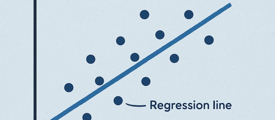
Linear Regression is one of the simplest and most common methods used in machine learning. Imagine you have a set of data points—like house prices versus sizes—and you want to find a straight line that best fits this data. The goal is to find a line that stays as close as possible to all the points on the plot. Once you’ve identified this line, it can be used to make predictions for new data.

For example, if you know the prices of houses with sizes 800 sqft, 1000 sqft, and 1200 sqft, Linear Regression helps you figure out the trend between size and price. With that trend, you can predict the price of a house that's 1100 sqft even if it isn’t part of the original data.

To break it down:

1. Plot the data points (size vs. price).

2. Draw the line that minimizes the distance from all the points (this is called "best fit").

3. Use this line to make predictions for other house sizes.
   For instance, based on your data, the model might predict that a house of size 1100 sqft costs $275,000.
   
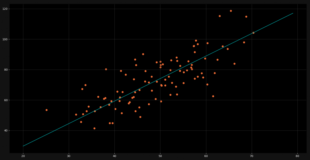
   As you can see we have a lot of orange data points. For every x-value we have a corresponding y-value. The linear regression line is right in between all of these points and gives us a good approximated y-value for ever x-value. However, linear models usually unfold their potential only in higher dimensions. There they are very powerful and accurate.

But how do we find this optimal regression line? Of course we could just use a machine learning library like Scikit-Learn, but this won’t help us to understand the mathematics behind this model. Because of that, in this tutorial we are going to code a linear regression algorithm in Python from scratch.

Perquisites

If we're building this algorithm from scratch, we'll use two handy data science tools: Pandas and Matplotlib. Pandas is great for importing and managing data in CSV files, making it easy for us to work with structured data. Matplotlib helps us visualize our model, like creating graphs or charts to understand the patterns and results better. These tools make our coding and analysis smoother and more effective! 😊

import pandas as pd
import matplotlib.pyplot as plt

Also it would be very beneficial for you to have a decent understanding of high school math and calculus. These are not inalienable for the programming but definitely for the understanding of the mathematics behind linear regression. You will need some basic knowledge about partial derivatives. But if you are just here for the code and you don’t care too much about the mathematics, you can go on as well.

Basics of Linear Regression

In the context of Linear Regression, the model assumes a linear relationship between the dependent variable
𝑦 = (output) and the independent variable
𝑥 = (input). The equation for a linear model is expressed as:
**𝑦=𝑚.𝑥+𝑏**
Where:

• 𝑚: Gradient (slope of the line), representing the rate of change in 𝑦 with respect to 𝑥.

• 𝑏: Intercept, representing the value of 𝑦 when 𝑥 = 0.

To determine 𝑚 and 𝑏, we need to optimize these parameters using the loss function and the gradient descent algorithm.

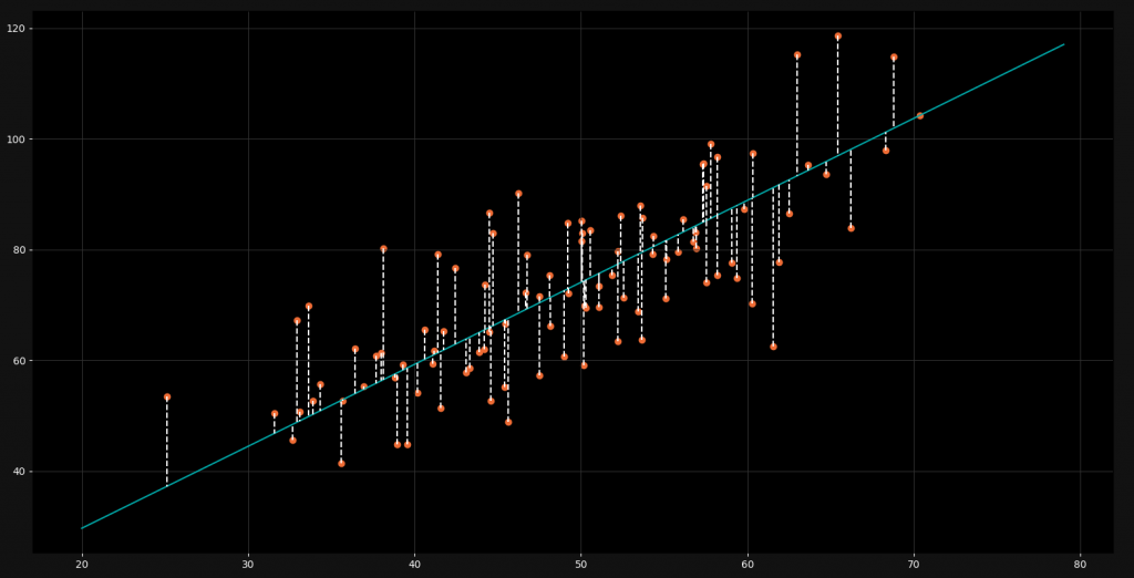
Loss Function

The loss function quantifies the error between the actual values (𝑦(true)) and the predicted values (𝑦(pred.)) from the model. A common choice is the Mean Squared Error (MSE), defined as:

MSE=1/n∑(𝑦(true)i - y(𝑝𝑟𝑒𝑑)i^2

Where:

• 𝑛: Number of data points
• 𝑦ₜᵣᵤₑ,𝑖: Actual value for the 𝑖ₜₕ data point
• 𝑦ₚᵣₑ𝑑,𝑖 = 𝑚 ⋅ 𝑥𝑖 + 𝑏: Predicted value for the 𝑖ₜₕ data point

The goal is to minimize the value of the loss function, meaning the model's predictions get as close as possible to the true values.

Implementing Linear Regression in Python

As I already mentioned in the beginning we will need the two libraries Matplotlib and Pandas for loading and visualizing the data.

import pandas as pd
import matplotlib.pyplot as plt

The next step is to load our data from a CSV-file into our script. For this tutorial we are using a simple file with some x-values and y-values.
example:

points = pd.read_csv('data.csv')

Now that we have our data in the script, we can start defining our functions. Let’s start with the loss function.

def loss_function(m, b, points):
    total_error = 0
    for i in range(len(points)):
        x = points.iloc[i, 0]
        y = points.iloc[i, 1]
        total_error += (y - (m * x + b)) ** 2
    return total_error / float(len(points))

To implement the mathematical principles of gradient descent, we iterate through each data point to compute the partial derivatives for 𝑚 (the gradient) and 𝑏 (the intercept). These derivatives indicate the steepness of the slope at each point, guiding the optimization process. After performing the calculations, the algorithm updates 𝑚 and 𝑏 with their new values, moving closer to the optimal solution. The learning rate plays a critical role here—it controls the magnitude of these updates, determining how significantly 𝑚 and 𝑏 are adjusted in each iteration. This iterative approach ensures gradual refinement, leading to an effective model.

Gradient Descent
Gradient descent is an optimization algorithm used to minimize a given function, often referred to as the "loss function," in machine learning and mathematics. Its purpose is to find the optimal parameters (e.g., coefficients in Linear Regression) that minimize the error between the predicted and actual values.
Detail Part next Blog

Now actually training the model is very easy. We just need to define some initial values and then apply our funciton.

m = 0
b = 0
L = 0.0001
epochs = 1000

for i in range(epochs):
    m, b = gradient_descent(m, b, points, L)

print(m, b)

To start optimizing our model using gradient descent, we initialize the two key parameters (𝑚 and 𝑏) to 0. These represent the slope and intercept of our linear equation.

Next, we define the learning rate (𝛼) as 0.0001—a small positive value that controls how much the parameters are adjusted during each iteration. This value is crucial, as a properly chosen learning rate ensures a smooth and stable optimization process.

The number of epochs is another important factor. It specifies how many times we repeat the gradient descent algorithm across the dataset. A higher number of epochs means more iterations, leading to finer-tuned parameters.

Finally, we run a loop that iterates through the dataset, computes the gradients (partial derivatives for 𝑚 and 𝑏), and updates their values iteratively. This process continues for the specified number of epochs, gradually minimizing the error and improving our model.

Output : 1.4934002376 0.08805678923

Thanks for reading...